Graphically analysing and statistically testing influence factors in a process

Imagine you have mapped a process and you have already identified possible influencing factors. The next step is to determine whether these factors really influence the process and how much influence they have. But how do you go about this?

Funnel of analysis of influence factors

You can compare analysing influence factors with a funnel: you start with a wide range of possibilities and gradually filter them down to a smaller group of real causes. First you exclude factors that clearly have no influence, then you examine the remaining factors more thoroughly. This process resembles the work of a detective who gathers clues and a judge who makes a judgment based on facts (Figure 1).

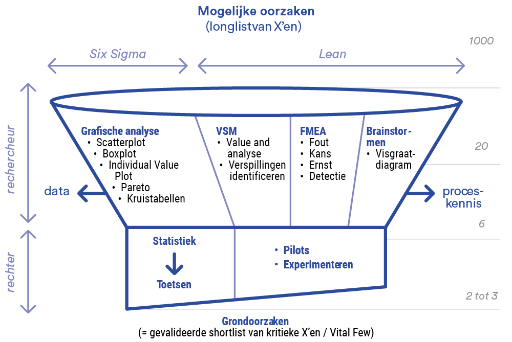
Figure 1: Funnel of analysis of influence factors

Process knowledge and data analysis

When identifying influencing factors, you use process knowledge on the one hand and data analysis on the other. If you have data available, you often start with visual analysis to identify patterns. Then you use statistical tests to determine whether the relationships you suspect actually exist. In this article, I discuss these two steps: graphic analysis and statistical tests.

Step 1: Graphical analysis - discovering patterns

To start, you determine which measurable aspects of the process affect performance. These become the Critical to Quality-aspects (CTQs) called.

Consider, for example, lead time, a commonly used process performance indicator. Then identify possible influencing factors, such as employee experience.

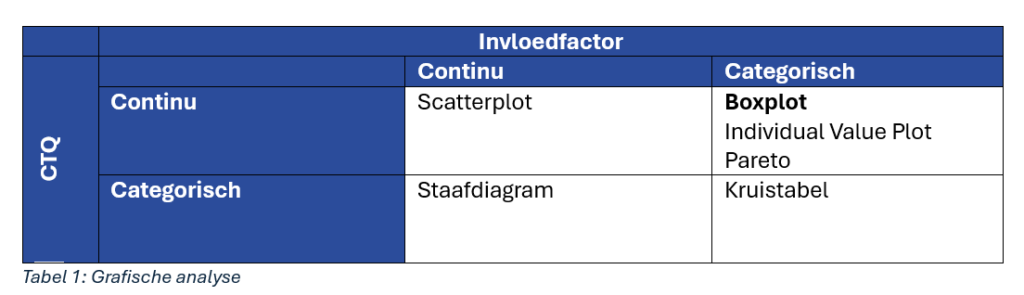
The data you collect can be continuous (e.g. lead time in minutes) or categorical (e.g. experience level: junior, medior or senior). Depending on the data type, you choose an appropriate graphical analysis method, such as a boxplot in this example (see table 1).

Example graphical analysis

Suppose you want to investigate whether employee experience affects lead time. With a boxplot, which visually displays group differences, you can quickly detect possible differences between groups. Figure 2 shows that junior employees tend to have longer turnaround times than medians and seniors, suggesting that experience plays a role.

Step 2: Statistical test - confirm correlations

After the graphical analysis, you may already have an idea whether there is a relationship between employee experience and turnaround time. But to be sure, you'll want to test this with a statistical test. Once you have identified patterns with graphs, you can use statistical tests to assess whether these links are actually significant.

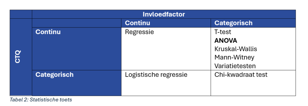
In the example, you use an ANOVA test, which compares group averages, because you want to analyse transit time (continuous data) in relation to different levels of experience (categorical data) (see table 2).

The analysis consists of two steps:

Checking assumptions: Before you can interpret the results of the ANOVA, check that the data meets the assumptions of the test. This includes, for example, a residuals analysis to assess whether the data is normally distributed and whether the variances between groups are equal.
Interpreting results: If the assumptions are valid, you analyse the group averages. With this, you determine whether there is a significant difference between experience levels with respect to lead time.

By following these steps, you can make statements about the relationship between experience and lead time with more certainty.

Note: check assumptions in statistical tests

Before applying a statistical test such as ANOVA, it is important to check that the data meets the necessary assumptions. For the ANOVA, this means, among other things, that the residuals should be normally distributed and that the variances between groups should be equal. If the data does not meet these assumptions, you can consider using an alternative test, such as the Kruskal-Wallis test. This non-parametric test has less stringent assumptions and is suitable for data that is not normally distributed.

Step 2a: Check assumptions - residual analysis

Before you can trust the ANOVA results, you check whether the data meets the assumptions, such as normality. You do this with a residuals analysis. Residuals are the differences between the observed values and the predicted values of the model. By analysing these residuals, you check whether they are randomly distributed and meet the normality assumptions.

In such a statistical test, you formulate two hypotheses:

The null hypothesis: The residuals are normally distributed.
The alternative hypothesis: The residuals are not normally distributed.

The p-value from the test gives the probability that you would observe a deviation from normality, if the null hypothesis is true. A p-value greater than 0.05 means that there is insufficient evidence to reject the null hypothesis. In other words, there is no strong indication that the residuals are not normally distributed. Therefore, we accept the null hypothesis in this case: the residuals are normally distributed.

In our example, the p-value is 0.343, which is greater than 0.05. This means that the probability of such deviation under the null hypothesis is large enough and the residuals meet the normality assumptions. This allows us to safely apply the ANOVA and consider the results reliable. As indicated earlier, if normality is not confirmed, you can consider alternative non-parametric tests, such as the Kruskal-Wallis test.

Step 2b: Interpret results - analysis of averages

The ANOVA test shows that there is a significant difference in processing times between the groups. In this test, you formulate two hypotheses:

The null hypothesis: There is no difference in average turnaround times between the groups (experience plays no role).
The alternative hypothesis: There is at least one group whose average turnaround time differs significantly (experience plays a role).

The p-value from the ANOVA test gives the probability of seeing the observed differences or larger differences in group averages, if the null hypothesis is true. When the p-value is smaller than 0.05, it means that the probability of such differences is very small under a correct null hypothesis. In that case, we reject the null hypothesis and accept the alternative hypothesis: there is a significant difference in turnaround times between the groups, and experience thus plays a role.

In our example, a p-value smaller than 0.05 confirms that experience actually has an effect on lead times. The explanation for this is based on process knowledge: junior employees often work under supervision, which can take extra time (Figure 3).

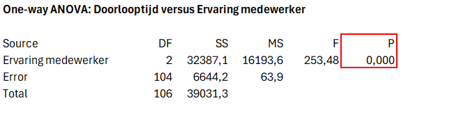
Figure 3: ANOVA results

Conclusion: visual and statistical evidence

By combining graphical analysis with statistical tests, you can not only visualise relationships, but also objectively determine whether they really exist. This allows you to make fact-based improvements to your process.